Unit 3: Substances and Mixtures

This unit connects particle-level structure (bonding within molecules and forces between them) to bulk properties (melting, boiling, solubility, conductivity) and to mixtures, especially solutions and gases. Ideas about polarity from Unit 2 carry directly into intermolecular forces and chromatography; moles and concentration from Unit 1 are key to the gas laws and colligative properties.

Intermolecular forces

Intermolecular forces (IMFs) are attractions between molecules or ions. They are much weaker than intramolecular (within a molecule) covalent or ionic bonds, but they control many everyday properties: boiling point, melting point, vapor pressure, surface tension, and solubility in a given solvent.

London dispersion forces

London dispersion forces arise from temporary electron fluctuations that create instantaneous dipoles, which in turn induce dipoles in neighbors. They are present in every substance (atoms and molecules). In nonpolar species they are often the only IMF and dominate cohesive energy. Strength grows with polarizability: larger electron clouds, higher molar mass in a homologous series, and greater surface area (e.g. linear versus branched alkanes) increase the amount of london disperson forces.

Dipole–dipole interactions

Polar molecules possess a permanent dipole moment, since the more electronegative element always tries to pull in electrons, creating a negatively-charged area around that element and a positive-charged area on the other element. Dipole–dipole attractions align partially positive ends toward partially negative ends. They are typically stronger than dispersion between comparable-sized molecules, though dispersion still contributes a little bit of force.

Hydrogen bonding

Hydrogen bonding is an especially strong dipole–dipole interaction (often treated as its own category) when hydrogen is bonded to F, O, or N: small, very electronegative atoms that leave a highly exposed proton. It explains the anomalously high boiling points of \(\text{H}_2\text{O}\), alcohols ( \(\text{-OH}\) ), and amines in appropriate contexts, since they all include hydrogen bonds.

Ion–dipole interactions

Ion–dipole forces act between an ion and the partial charges of a polar solvent. They are central to dissolving ionic compounds in water and are typically stronger than neutral-molecule IMFs, and therefore these are usually the strongest type of IMF.

Molecular polarity and physical properties

Bond polarity compares electronegativity across a bond; molecular polarity is the vector sum of bond dipoles in three dimensions. Symmetric molecules (e.g. \(\text{CO}_2\), \(\text{CCl}_4\)) can be nonpolar even with polar bonds because dipoles cancel. Lone pairs change geometry (VSEPR), which changes whether dipoles cancel, so lone pairs matter indirectly even though polarity is a property of the whole molecule, not “of” a lone pair in isolation. A good way to tell if a molecule is polar if its dipoles are not symmetrical, or if one dipole is significantly stronger than another.

Trends: among similar molecules, greater polarity and stronger IMFs tend to raise boiling point and lower vapor pressure; the opposite trend holds for weaker IMFs.

Different Solids and Properties

Selected bulk properties

Electrical conductivity is the ability for a substance to conduct electricity, basically meaning they have an active flow of electrons going through
Malleability and ductility describe the ability to deform without brittle fracture
Viscosity is a liquid’s resistance to flow; it rises with stronger IMFs and often with molecular size or hydrogen bonding
Crystalline solids have long-range order and often show sharp melting points. Amorphous solids (many glasses) lack that order and soften over a temperature range rather than melting at a single temperature.

Types of crystalline solids

Chemists often classify solids by the particles at lattice sites and the forces holding them together.

Ionic solids combine cations and anions in a regular crystal lattice. They tend to have high melting points, are brittle, conduct when molten or dissolved (mobile ions), and often dissolve in polar solvents. Ionic solids can be hydrated (water in the crystal, often written with \(\cdot\, x\,\text{H}_2\text{O}\) in the formula) or anhydrous (no water in the lattice). Ionic compounds are not described as “polar molecules” because they are not discrete polar molecules in the solid; they dissociate into ions in water.
Molecular solids are composed of discrete molecules held by IMFs. They are usually softer, lower-melting, and do not conduct as pure solids. Molecular solids are either polar or nonpolar, based on the distribution of dipoles.
Covalent network solids (e.g. diamond, quartz) extend covalent bonding through a three-dimensional network. They are typically very hard, high-melting, and insoluble (Exception: graphite is a network solid that conducts along planes).
Metallic solids feature cations in a sea of delocalized electrons, giving variable melting points, conductivity, and malleability. They look and feel metallic, so if a solid looks like a traditional metal, it is probably a metallic solid.

Identifying the type of solid

The main crystalline types behave differently in simple tests, so a short flowchart can narrow down the classification. Real samples can blur categories, so it is important to do many tests as backups.

Heating in a test tube: Look first for condensation near the cool top of the tube. Water driven off from a crystal can indicate a hydrated ionic solid (often you are done after also checking conductivity in water). If there is no such hint and the sample melts at modest temperature, it is likely a molecular or metallic solid; test electrical conductivity on the solid (and again if you have a melt): metallic solids conduct; molecular solids do not. Many ionic salts do not melt cleanly over a burner, they may sit unchanged or decompose, so “does not melt” is not enough to prove molecular.
Solid conductivity: If the solid conducts electricity, it is metallic (or graphite, a special network solid). If it does not conduct and you already know it melts easily, treat it as molecular and go to tests 4–5.
Aqueous Conductivity: If the solid does not dissolve, skip this step for now. If the solution conducts well, the solid is almost certainly ionic (anhydrous or hydrated—combine with step 1). If the solid dissolves but the solution does not conduct (or only very weakly), it is a molecular nonelectrolyte, usually polar (e.g. sugar). This step does not distinguish polar from nonpolar if the solid is insoluble in water.
Water solubility (for molecular solids): Use only when you have already ruled out metallic and ionic behavior. Dissolves in water → polar molecular (for typical neutral molecules). Does not dissolve in water → likely nonpolar molecular, but covalent network solids such as diamond or quartz are also insoluble and non-conducting; they usually do not melt in a test tube and are extremely hard—unlike most molecular crystals.
Hexane solubility (confirmation for molecular solids): Hexane is nonpolar. If the solid dissolves in hexane, it behaves like a nonpolar species (nonpolar molecular). If it does not dissolve in hexane but did dissolve in water, that matches polar molecular. If it dissolves in neither, reconsider ionic (if it never dissolved), network covalent, or a very high–molar-mass molecular solid.

Caveat: Covalent network solids are easy to confuse with nonpolar molecular solids in water/hexane tests alone: hardness, melting behavior, and structure from other evidence matter.

Separating mixtures

Chromatography separates components by differential affinity for a mobile phase and a stationary phase based on their differing polarity. It is typically done on cellulose or silica based paper (both polar) and involves dipping the bottom of the paper in a solvent (that is both polar and nonpolar) which allows the components to separate.

The retention factor is

\[R_f = \frac{\text{distance traveled by the spot}}{\text{distance traveled by the solvent front}},\]

with values between \(0\) and \(1\) for typical thin-layer work. The retention factor is a measure of how far a molecular moved compared to the solvent, and can determine the polarity of the molecule. Usually (if using polar paper and a polar stationary phase) nonpolar molecules will go higher than polar molecules, since they have a weaker attachment to the paper and thus will move up with the solvent more.

Other methods of separation include distillation (uses differences in boiling point (hence vapor pressure)) and evaporation/crystallization (removes or concentrates solvent to isolate solute).

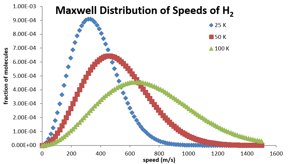
Temperature, kinetic energy, and the Maxwell–Boltzmann distribution

Temperature (in Kelvin) is proportional to the average translational kinetic energy of ideal-gas molecules, but varies per molecule. However, the KE can be mapped as a distribution (called the Maxwell-Boltzmann distribution). A Maxwell–Boltzmann curve plots fraction versus speed or energy. Lighter gases at the same \(T\) have higher average speed, and raising \(T\) broadens the curve and increases the fraction with energy above a given activation energy. Note that macroscopic kinetic energy \(\frac{1}{2}mv^2\) applies to bulk motion; do not confuse it with thermal motion of molecules inside a sample. An example of a Maxwell-Boltzmann distribution can be seen below:

Maxwell Boltzmann Distribution

Kinetic molecular theory

Kinetic molecular theory sets down some assumptions for an ideal gas:

The gas molecules have negligible volume compared to the container
The gas molecules have no IMFs
The gas molecules perform elastic collisions with each other and the walls of the container
The gas molecules move around in constant, random motion
For one mole of a monatomic ideal gas, average translational kinetic energy (per mole) is

\[KE_{avg} = \frac{3}{2}RT.\]

Per molecule, the equation becomes \(KE_{avg} = \frac{3}{2} k_B T\)

with Boltzmann’s constant \(k_B = 1.38 \times 10^{-23} \text{ J/K}\). Temperature in this model is proportional to the mean kinetic energy of random motion. In addition, if you are solving for velocity, the average RMS (root mean square, one way to taking an average) speed of the molcules is:

\[v_{RMS} = \sqrt{\frac{3RT}{M}}.\]

Always remember that kinetic energy is distributed along a Maxwell-Boltzmann distribution, so we always talk about the average kinetic energy and RMS velocity.

Pressure, STP, and the Ideal Gas Law

Pressure measures force per unit area. Useful conversions include

\[1 \text{ atm} = 760 \text{ mmHg} = 760 \text{ torr} = 101.325 \text{ kPa} = 14.7 \text{ psi} = 1.013 \text{bar}\]

STP (standard temperature and pressure) is commonly taken as \(0^\circ\text{C}\) (\(273.15 \text{ K}\)) and \(1 \text{ atm}\), with one mole of an ideal gas under those conditions occupies about \(22.4 \text{ L}\) (Modern IUPAC defines a slightly different standard pressure, but for AP chemistry purposes this is the standard pressure). For the remainder of the unit and AP Chemistry, we will use the following notations, along with their standard units:

\(P\) = pressure (in atm, mmHg, torr, kPa, bar, or psi)
\(V\) = volume (L)
\(n\) = number of moles (mol)
\(T\) = temperature (Kelvin)

The Gas Laws and the Ideal Gas Law

There are many gas laws that are useful for the AP exam (Remember to ALWAYS use Kelvin!):

Boyle’s law: \(P_1 V_1 = P_2 V_2\) (or equivalently \(P \propto \frac{1}{V}\)) at fixed \(n\) and \(T\).
Charles’s law: \(\frac{V_1}{T_1} = \frac{V_2}{T_2}\) (or equivalently \(V \propto T\)) at fixed \(n, P\) (use Kelvin for \(T\)).
Gay-Lussac’s law: \(\frac{P_1}{T_1} = \frac{P_2}{T_2}\) (or equivalently \(P \propto T\)) at fixed \(n\) and \(V\).
Avogadro’s law: \(\frac{V_1}{n_1} = \frac{V_2}{n_2}\) (or equivalently \(V \propto n\)) at fixed \(P\) and \(T\).

The combined gas laws can merge to form the Ideal Gas Law (IGL):

\[PV = nRT.\]

Use a value of \(R\) whose pressure and volume units match the problem:

\[R = 0.08206\ \text{L}\cdot\text{atm}/(\text{mol}\cdot\text{K})\]
\[R = 8.314\ \text{J}/(\text{mol}\cdot\text{K}) = 8.314\ \text{kPa}\cdot\text{L}/(\text{mol}\cdot\text{K})\]
\[R = 62.36\ \text{L}\cdot\text{torr}/(\text{mol}\cdot\text{K})\]
\[R = 0.08314\ \text{L}\cdot\text{bar}/(\text{mol}\cdot\text{K})\]

Molarity in the gas phase is often written \(C = n/V\), giving

\[P = CRT\]

for an ideal gas at temperature \(T\).

Two useful rearrangements combine the ideal gas law with molar mass \(M\):

\[d = \frac{PM}{RT}\]

for gas density \(d\), and

\[M = \frac{dRT}{P}\]

when density is measured directly. These are just \(PV=nRT\) with \(n=m/M\) and \(d=m/V\).

Dalton’s law of partial pressures: for a mixture of ideal gases,

\[P_{\text{total}} = \sum P_i, \qquad P_i = x_i P_{\text{total}},\]

where \(x_i\) is the mole fraction of gas \(i\). When collecting a gas over water, include the vapor pressure of water:

\[P_{\text{total}} = P_{\text{gas}} + P_{\text{H}_2\text{O}}.\]

Diffusion and effusion

Diffusion is mixing driven by random molecular motion, while effusion is escape through a small opening. Graham’s law compares rates for gases at the same temperature:

\[\frac{\text{rate}_1}{\text{rate}_2} = \sqrt{\frac{M_2}{M_1}},\]

where \(M\) is molar mass. Graham’s Law basically states that lighter molecules move faster on average and effuse faster.

Real gases

Real gases deviate when volume is finite and attractions matter. The van der Waals equation is a textbook correction:

\[\left(P + \frac{an^2}{V^2}\right)(V - nb) = nRT.\]

The compressibility factor is a measure of the effects of IMFs on a gas:

\[Z = \frac{PV}{nRT}\]

which equals \(1\) for an ideal gas (by Ideal Gas Law). \(Z < 1\) often reflects attractive effects dominating at moderate pressure, and \(Z > 1\) can appear when repulsive effects dominate at high pressure. Note that this is not very important for an AP context.

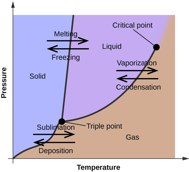
Phase behavior and phase diagrams

Vapor pressure is the pressure of vapor in equilibrium with a condensed phase at a given temperature; it rises with \(T\) and reflects IMF strength (volatile liquids have high vapor pressure at a given \(T\)). A phase diagram plots pressure versus temperature; the triple point is where solid, liquid, and gas coexist. The critical point ends the liquid–vapor boundary; above the critical temperature there is no distinct liquid phase at any pressure.

Phase Diagram

Colligative properties of solutions

Colligative properties depend on the concentration of solute particles, not on their chemical identity. When you dissolve a solid into a liquid, it increases the IMFs/interactions between the molecules. Resulting in the following formulas (Use molality \(m\) (moles solute per kilogram solvent) in the standard formulas):

Boiling point elevation:

\[\Delta T_b = i K_b m.\]

Freezing point depression:

\[\Delta T_f = i K_f m.\]

\(K_b\) and \(K_f\) are solvent constants. The van’t Hoff factor \(i\) is the moles of dissolved particles produced per mole of formula units added (for molecular solids \(i = 1\)). Although this is not always the case, for ionic solids, you can assume that \(i\) is the number of ions that result after one molecule of the solid dissolves.

Vapor pressure of solutions and volatile mixtures

All liquids tend to evaporate, since their energy can be mapped to a Maxwell-Boltzmann distribution. The pressure generated by the evaporation is called vapor pressure. Raoult’s law for a nonvolatile solute states that:

\[P_{\text{solution}} = x_{\text{solvent}}\, P^\circ_{\text{solvent}},\]

lowering vapor pressure relative to the pure solvent. For two volatile components,

\[P_{\text{total}} = x_A P^\circ_A + x_B P^\circ_B\]

when the mixture is ideal. Positive deviations from Raoult’s law mean weaker attractions between unlike molecules than the average of like–like interactions; negative deviations mean stronger attractions between unlike partners.

Henry’s law relates gas solubility in a liquid to partial pressure:

\[C = k_H P,\]

with \(k_H\) a constant for a given solute–solvent pair at fixed \(T\).

Osmotic pressure

For dilute solutions, osmotic pressure \(\Pi\) obeys

\[\Pi = i M R T,\]

with \(M\) in \(\text{mol/L}\) and \(R\) matched to the units of \(\Pi\) (commonly \(0.0821 \text{ L}\cdot\text{atm}/(\text{mol}\cdot\text{K})\) when \(\Pi\) is in atm). Osmosis is net flow of solvent through a semipermeable membrane toward higher solute concentration. Note that this will likely not appear on the AP Chemistry exam.

Light and solutions: Beer–Lambert law

Spectrophotometry/colorimetry uses the Beer–Lambert Law (Or alternatively Beer’s Law): absorbance is proportional to concentration for a fixed path length:

\[A = \varepsilon l c,\]

where \(\varepsilon\) is the molar absorptivity, \(l\) the path length, and \(c\) the concentration. Transmittance \(T\) (fraction of light passing) relates to absorbance by

\(A = -\log_{10}(T)\),

but transmittance rarely shows up on the AP exam. Beer’s law is very applicable for measuring equilibrium/kinetics, since absorbance is directly proportional to concentration. When doing colorimetry, always calibrate beforehand and set the wavelength to the wavelength that is closest to the OPPOSITE of the color of the solution to get maximum absorbance.