Unit 7: Equilibrium
Unit 7 is about chemical equilibrium: the state in a closed system where a reversible reaction’s forward and reverse rates are equal, so macroscopic concentrations (or partial pressures) stop changing even though reactants and products are still interconverting at the molecular level. You will write equilibrium constants (\(K_c\), \(K_p\)), compare them to the reaction quotient (\(Q\)), use ICE tables to compute equilibrium compositions, apply Le Châtelier’s principle to predict disturbance responses, and extend the same ideas to solubility (\(K_{sp}\)), precipitation, and complex-ion formation (\(K_f\)). These tools connect directly to thermodynamics through Gibbs free energy and the van’t Hoff equation (how \(K\) changes with temperature), and to later work on acids and bases, where \(K_a\) and \(K_b\) are themselves equilibrium constants.
Chemical Equilibrium
Most reactions we have looked at previously were irreversible reactions, or reactions that can only go one way (forward). A reversible reaction can run in both directions (forward and backwards). In a closed system (no escape of matter), the forward reaction consumes reactants and forms products, while the reverse reaction does the opposite. Chemical equilibrium is reached when the rate of the forward reaction equals the rate of the reverse reaction. At that point:
- Concentrations (or for gases, partial pressures) remain constant over time (they are not necessarily equal to one another)
- The system is dynamic: molecules still react, but there is no net change in amounts. This is different from a completed or irreversible reaction, where at least one reactant is effectively exhausted and the process does not establish a lasting balance between forward and reverse paths at ordinary conditions.
Homogeneous equilibrium means all reacting species are in the same phase (e.g. all gases, or all in one solution). Heterogeneous equilibrium includes pure solids or pure liquids as separate phases; their activities are taken as constant and they are omitted from the equilibrium expression (see below).
Equilibrium constant \(K_c\)
For a balanced reaction in solution (molar concentrations in \(\text{mol/L}\)),
\[j\text{A} + k\text{B} \rightleftharpoons l\text{C} + m\text{D},\]the equilibrium constant in terms of concentration is
\[K_c = \frac{[\text{C}]^l [\text{D}]^m}{[\text{A}]^j [\text{B}]^k},\]where each \([]\) is the equilibrium molarity raised to the power of the stoichiometric coefficient. Only aqueous solutes or gases appear in \(K_c\), since the concentrations of pure solids/liquids do not change, and therefore are always assumed to be 1. In addition, \(K_c\) will not change unless temperature changes, so \(K_c\) is only temperature-dependent.
On the AP exam, \(K\) is treated as a dimensionless ratio by implicitly comparing each concentration to a standard reference (standard state). Regardless, you should still use the same algebraic form when you set up problems.
Extreme \(K_c\) value rules
Orders of magnitude help you judge extent (at a given temperature):
- If \(K_c\) is very large (e.g. \(K_c \gg 1\), sometimes textbook thresholds like \(K_c > 10^{10}\)), the forward reaction is product-favored at equilibrium—substantial conversion to products. This usually means that the forward reaction is approximately an irreversible reaction
- If \(K_c\) is very small (e.g. \(K_c \ll 1\), sometimes \(K_c < 10^{-10}\)), the mixture stays reactant-heavy, meaning that the reaction basically did not start at all.
These cutoffs are rules of thumb; what matters is comparing \(Q\) to \(K\) and interpreting \(K\) relative to \(1\).
Manipulating \(K\) for related equations
- Reverse reaction:
\(K_{c,\text{reverse}} = \frac{1}{K_{c,\text{forward}}}.\) - Multiply the whole equation by an integer \(n\):
\(K_c' = (K_c)^n\) - Add sequential steps (all at the same temperature): the overall \(K\) is the product of the step constants:
\(K_{\text{overall}} = K_1 \times K_2 \times \cdots\)
Equilibrium in the gas phase: \(K_p\)
For gas-phase equilibria it is often convenient to use partial pressures (in atmospheres on the AP exam, unless stated otherwise). For
\[j\text{A}(g) + k\text{B}(g) \rightleftharpoons l\text{C}(g) + m\text{D}(g),\]define
\[K_p = \frac{(P_{\text{C}})^l (P_{\text{D}})^m}{(P_{\text{A}})^j (P_{\text{B}})^k}.\]Only gaseous species appear (since aqueous solutions and pure solids/liquids do not have partial pressures). From the ideal gas law, \(P = (\text{n/V})RT = MRT\) for a gas (M = molarity). The standard relationship is
\[K_p = K_c (RT)^{\Delta n_{\text{gas}}},\]where \(\Delta n_{\text{gas}}\) is difference between the amount of moles of products and reactants (from the balanced equation), and \(R\) must be consistent with the pressure units used (e.g. \(R = 0.0821\ \text{L·atm/(mol·K)}\) when \(P\) is in atm).
Reaction quotient \(Q\)
The reaction quotient has the same algebraic form as \(K\), but it uses concentrations or pressures at any instant, not necessarily at equilibrium.
For concentrations:
\[Q_c = \frac{[\text{C}]^l [\text{D}]^m}{[\text{A}]^j [\text{B}]^k}.\]Interpreting \(Q_c\) vs \(K_c\)
- If \(Q < K\), the ratio of products to reactants is too small for equilibrium; the system shifts right (toward products).
- If \(Q > K\), the ratio is too large; the system shifts left (toward reactants).
- If \(Q = K\), the system is at equilibrium.
A useful trick is to line up \(K\) and \(Q\) alphabetically (so \(K\) on the left and \(Q\) on the right), and whatever direction the sign goes (e.g. < (less than) goes left) is the direction the reaction goes.
The same logic applies to \(Q_p\) and \(K_p\) for gases.
A catalyst speeds both forward and reverse rates equally, so it does not change \(K\) or the equilibrium position - it only shortens the time needed to reach equilibrium.
Gibbs free energy and equilibrium
The link between standard Gibbs free energy change and the equilibrium constant (same temperature) is
\[\Delta G^\circ = -RT \ln K,\]where \(K\) is \(K_c\) or \(K_p\) according to how the reaction is expressed, and must match the standard-state convention your course uses. For many AP problems, \(K\) is \(K_c\) for solution chemistry and \(K_p\) when all species are gases and the expression is written in pressures. The Gibbs free energy value determines if a reaction is spontaneous, which is talked about more in Unit 9.
Qualitative connections (at standard conditions, using \(K\) relative to \(1\)):
- If \(K > 1\), then \(\Delta G^\circ < 0\): the forward reaction is thermodynamically favorable (spontaneous) under standard conditions.
- If \(K < 1\), then \(\Delta G^\circ > 0\): the reverse direction is favored under standard conditions and the forward reaction is not spontaneous.
- If \(K = 1\), then \(\Delta G^\circ = 0\), meaning the reaction is at equilibrium.
For nonstandard conditions, the reaction quotient enters:
\[\Delta G = \Delta G^\circ + RT \ln Q.\]At equilibrium, \(Q = K\) and \(\Delta G = 0\), which recovers \(\Delta G^\circ = -RT \ln K\). Here \(R\) is the gas constant (\(8.314\ \text{J/(mol·K)}\) when using joules), and \(T\) is kelvin.
The van’t Hoff equation
Le Châtelier’s principle says that \(K\) changes with temperature only, and the van’t Hoff equation makes that dependence quantitative. It follows from the way \(\Delta G^\circ = -RT\ln K\) combines with \(\Delta G^\circ = \Delta H^\circ - T\Delta S^\circ\) when you ask how \(K\) must move if \(T\) changes (treating \(\Delta H^\circ\) and \(\Delta S^\circ\) as approximately constant over a modest temperature range: a standard AP assumption unless a problem says otherwise).
If \(K_1\) and \(K_2\) are equilibrium constants (same kind: both \(K_c\) or both \(K_p\), matching how the reaction is written) at absolute temperatures \(T_1\) and \(T_2\), then
\[\ln\frac{K_2}{K_1} = -\frac{\Delta H^\circ}{R}\left(\frac{1}{T_2}-\frac{1}{T_1}\right) = \frac{\Delta H^\circ}{R}\left(\frac{1}{T_1}-\frac{1}{T_2}\right).\]Here \(\Delta H^\circ\) is the standard enthalpy change for the reaction as written (see Unit 6: Thermochemistry). Use \(R = 8.314\ \text{J/(mol·K)}\) when \(\Delta H^\circ\) is in joules per mole of reaction as written.
Sign check: if the forward reaction is endothermic (\(\Delta H^\circ > 0\)) and \(T_2 > T_1\), then \(K_2 > K_1\)—warming increases \(K\), matching the picture that heat acts like a reactant in an endothermic forward process. If the forward reaction is exothermic (\(\Delta H^\circ < 0\)), raising \(T\) decreases \(K\).
The differential form (useful conceptually and in derivations) is
\[\frac{d\ln K}{dT} = \frac{\Delta H^\circ}{RT^2},\]which shows that sensitivity of \(\ln K\) to temperature is larger when \(\Delta H^\circ\) is large and when \(T\) is low (through the \(1/T^2\) factor in how small \(\Delta T\) steps accumulate).
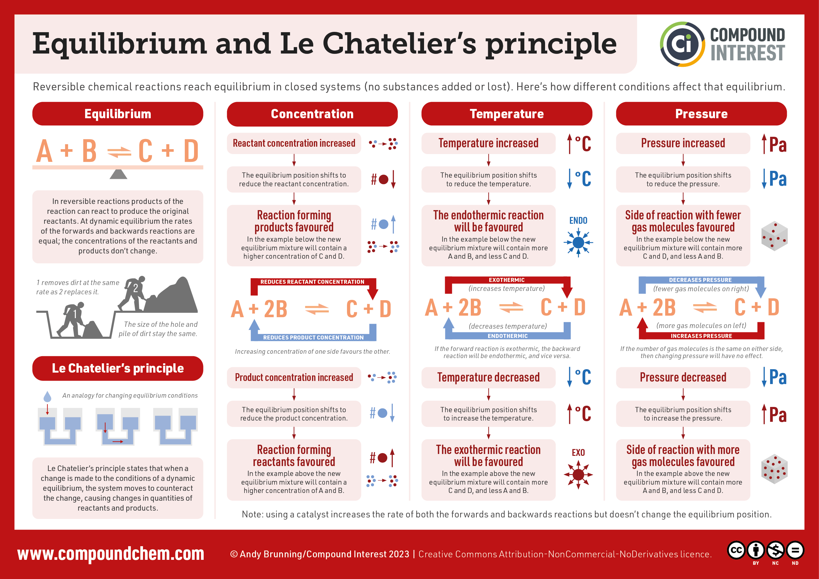
Le Châtelier’s principle
Le Châtelier’s principle is a qualitative rule: if a stress disturbs an equilibrium, the system shifts in the direction that partially counteracts the stress (new equilibrium is established; \(K\) is unchanged unless temperature changes).
Typical stresses:
- Concentration: Adding a reactant shifts toward products; removing a product does the same. Adding product shifts toward reactants.
- Pressure (gases): Reducing volume increases total pressure; the system shifts toward the side with fewer moles of gas (if any). Adding an inert gas at constant volume does not change partial pressures of reactants/products—no shift. At constant pressure, adding inert gas increases volume and can shift the equilibrium; AP questions usually emphasize the constant-volume case.
- Temperature: \(K\) changes with temperature. Treat heat as part of the reaction: for an endothermic forward reaction (\(\Delta H > 0\)), raising \(T\) favors the forward direction (larger \(K\) if the forward reaction is endothermic). For an exothermic forward reaction (\(\Delta H < 0\)), raising \(T\) favors the reverse direction (smaller \(K\)). Cooling favors the exothermic direction.
Since \(K\) depends on \(T\), do not treat temperature like a simple concentration stress when you need a numerical \(K\): use the correct \(K\) for the new temperature if given, compute \(K_2\) from \(K_1\) with the van’t Hoff equation (previous section), or reason qualitatively from \(\Delta H\).
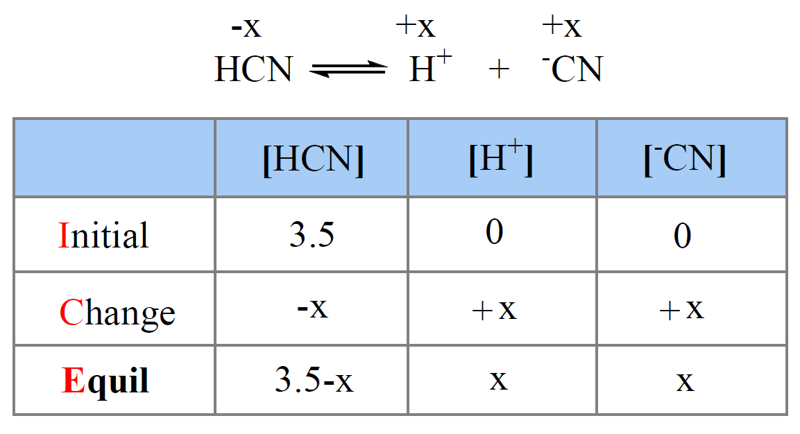
ICE tables
ICE stands for Initial, Change, Equilibrium. You use a table to organize amounts (or concentrations) for one reversible process.
Setup:
- Write a balanced equation.
- Initial row: given starting concentrations (after any mixing).
- Change row: express unknown change as \(x\) (or a multiple like \(2x\) from stoichiometry): reactants lose (\(-jx\), etc.) and products gain (\(+lx\), etc.), although you could swap the signs and have the same result. Note that if one side is 0, it can’t lose any concentration, so it must have a positive change!
- Equilibrium row: Initial + Change.
Rules and tips:
- Omit pure solids and pure liquids from the table if they do not define the solution volume.
- If a reactant is limiting, one species may be consumed completely before equilibrium in a sequential sense; still check whether the reaction can proceed in reverse from that state (ICE applies to the equilibrium stage you model).
- Small \(K\) (product-poor): equilibrium lies left; \(x\) may be negligible compared to initial concentrations—verify with the 5% rule (or exact quadratic) when your course allows.
- Large \(K\): equilibrium lies right; sometimes you assume complete reaction first, then back-react a small amount.
Solubility equilibrium and \(K_{sp}\)
You might remember the solubility rules from Unit 4. For a sparingly soluble ionic solid (basically anything that is considered “insoluble” to water), dissolution is an equilibrium. For example,
\[\text{A}_m\text{B}_l(s) \rightleftharpoons m\,\text{A}^{a+}(aq) + l\,\text{B}^{b-}(aq).\]The solubility product is
\[K_{sp} = [\text{A}^{a+}]^m [\text{B}^{b-}]^l.\]The solid (precipitate) does not appear in \(K_{sp}\). This is equivalent to \(K_c\) but for a dissolution.
Setting up ICE tables for \(K_{sp}\)
Setting up an ICE table for \(K_{sp}\) is slightly different from a normal ICE table procedure.
Setup:
- Write a balanced equation for solubility (remember that the solid is ALWAYS on the left side).
- Initial row: given starting concentrations (after any mixing). For the concentration of the solid, just write “solid” in that box.
- Change row: This is the same as a regular ICE table.
- Equilibrium row: This is the same as a regular ICE table, except write “solid” for initial for the precipitate.
Molar solubility
Molar solubility (\(s\)) is the number of moles of solid that dissolve per liter of solution to reach saturation (under stated conditions). If one formula unit of \(\text{A}_m\text{B}_l\) produces \(m\) ions of \(\text{A}\) and \(l\) ions of \(\text{B}\), then at saturation
\[[\text{A}^{a+}] = ms, \qquad [\text{B}^{b-}] = ls,\]and
\[K_{sp} = (ms)^m (ls)^l = m^m\, l^l\, s^{m+l}.\]Solve for \(s\) given \(K_{sp}\), or \(K_{sp}\) given \(s\). In an ICE table, the molar solubility is equivalent to the \(x\) value.
Ion product and precipitation
The ion product \(Q_{sp}\) uses current ion concentrations in the \(K_{sp}\) expression (same form as \(K_{sp}\)).
- If \(Q_{sp} < K_{sp}\), the solution is unsaturated; more solid can dissolve.
- If \(Q_{sp} = K_{sp}\), the solution is saturated (at equilibrium with solid, if present).
- If \(Q_{sp} > K_{sp}\), precipitation occurs until \(Q_{sp}\) drops to \(K_{sp}\) (assuming equilibrium can be reached).
Common-ion effect
If one of the ions is already present from another source (common ion), its higher initial concentration shifts dissolution left, lowering molar solubility compared to pure water. ICE-style reasoning applies: treat initial \([\text{A}^{a+}]\) or \([\text{B}^{b-}]\) as nonzero before the solid dissolves further.
Selective precipitation
Selective precipitation separates ions by adding a reagent that forms salts with very different \(K_{sp}\) values. The ion whose \(Q_{sp}\) exceeds its \(K_{sp}\) first (lowest \(K_{sp}\) or favorable stoichiometry) precipitates preferentially as concentration is raised—used analytically and conceptually on the exam.
Complex ions and formation constants
A complex ion consists of a central metal cation (Lewis acid) bound to ligands (Lewis bases) that donate electron pairs (learn more about acids/bases in Unit 8). In a solution, stepwise binding equilibria exist; textbooks often emphasize an overall formation (stability) constant \(K_f\) for
\[\text{M}^{n+} + x\,\text{L} \rightleftharpoons \text{ML}_x^{n+},\]with
\[K_f = \frac{[\text{ML}_x^{n+}]}{[\text{M}^{n+}][\text{L}]^x},\]matching the form of \(K_c\) for that net reaction (charges and stoichiometry depend on the specific complex). A larger \(K_f\) means the complex is more stable (more product-favored at equilibrium). If ligand is in large excess and \(K_f\) is large, it is often reasonable to assume complete formation for stoichiometry purposes—check problem assumptions.
The dissociation constant \(K_d\) for breaking the complex apart is the reciprocal of \(K_f\) for the same net forward/back pairing:
\[K_f = \frac{1}{K_d}.\]Coordination number is the number of donor atoms bound to the metal; common geometries include linear (2), tetrahedral or square planar (4), and octahedral (6).
Working checklist for problems
- Balance the equation and identify phase of each species.
- Write \(K_c\), \(K_p\), or \(K_{sp}\) omitting pure solids/liquids (and solvent water in dilute aqueous \(K_c\) unless specified).
- Compute \(Q\) if asked whether the system shifts; compare to \(K\).
- Use ICE for unknown equilibrium concentrations; watch stoichiometric multiples of \(x\).
- Remember temperature changes \(K\); catalyst does not. For two temperatures, relate \(K_1\) and \(K_2\) with the van’t Hoff equation if \(\Delta H^\circ\) is known (or given).
- For solubility, track common ions, \(Q_{sp}\) vs \(K_{sp}\), and complex formation, which can increase solubility by tying up a metal ion (e.g. \(\text{AgCl}\) dissolving more in ammonia).
This unit’s equilibrium constant logic is the same machinery you will reuse for acid–base (\(K_a\), \(K_b\), \(K_w\)) and buffers in the next unit—only the chemical reaction and symbols change.